Traditional audio processing pipelines rely on the Short-Time Fourier Transform (STFT) to convert waveforms into spectrograms. The STFT uses a fixed set of sinusoidal basis functions — which means the frequency resolution is baked in at design time. iSincNet takes a different approach: it replaces the fixed STFT with a learnable filterbank based on parametric sinc functions, producing a spectrogram representation that can be jointly optimized with downstream tasks.
This post walks through the encoder and decoder architecture. The key insight is that the entire encoding step can be written as a single matrix multiplication, making it both interpretable and fast.
Examples
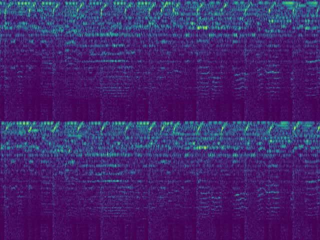
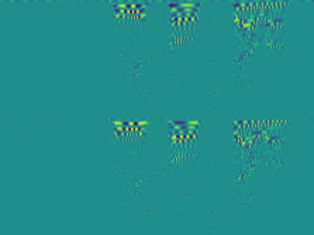
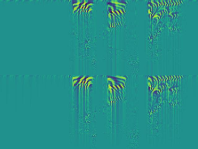
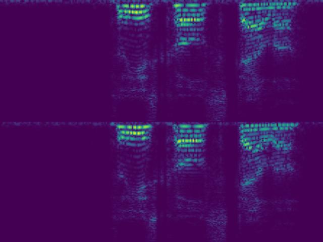
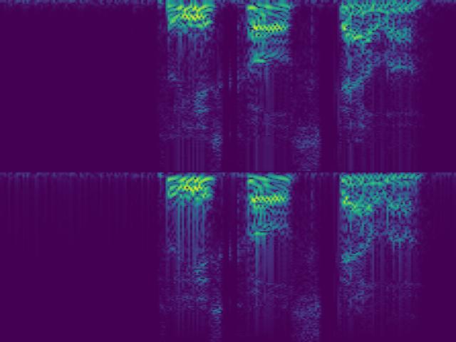
Before diving into the math, here are two audio samples and their corresponding SincNet spectrograms. Each sample is shown in four variants: signed vs. absolute value, and causal vs. non-causal encoder.
Music — Space of Souls (DJ Max)

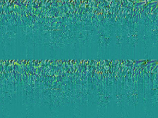
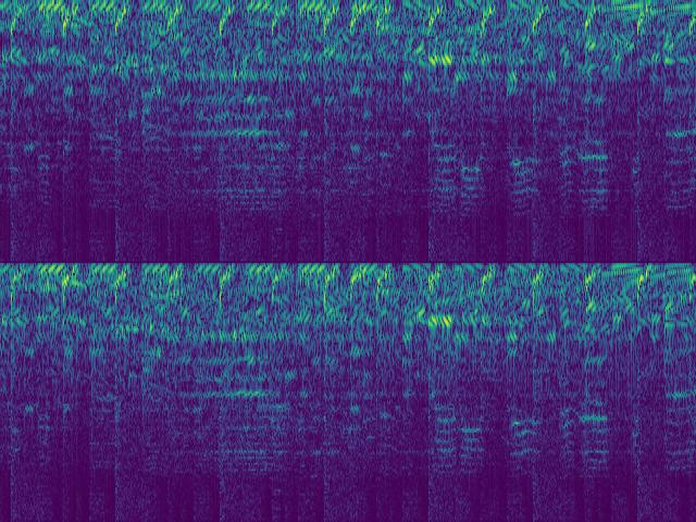
Speech
Encoder
The encoder transforms a raw audio waveform into a 2D spectrogram. The process has two steps: split the waveform into overlapping chunks, then pass each chunk through a bank of learned filters.
Chunking the waveform
Given a discrete waveform $x \in \mathbb{R}^{N}$, we extract overlapping frames of length $K$ with a hop size $H$. This produces $T = \lfloor (N - K) / H \rfloor + 1$ frames, which we stack column-wise into a matrix:
$$\mathbf{X} \in \mathbb{R}^{K \times T}$$Each column $\mathbf{X}_{:,t}$ is a windowed segment of the original signal centered at time $t$. This is identical to what the STFT does before applying the Fourier basis — the difference is what comes next.
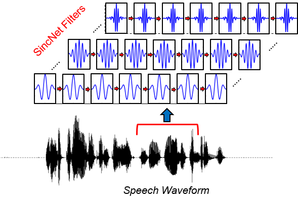
The filterbank
Instead of using fixed sinusoidal basis functions, iSincNet uses a bank of $F$ parametric bandpass filters. Each filter $h_f$ is defined as the difference of two sinc functions:
$$h_f[n] = 2 f_2 \, \text{sinc}(2 f_2 n) - 2 f_1 \, \text{sinc}(2 f_1 n)$$where $f_1$ and $f_2$ are the learnable low and high cutoff frequencies of the $f$-th filter. These parameters are the only things being learned — two scalars per filter. We stack all $F$ filters row-wise into a filter matrix:
$$\mathbf{W} \in \mathbb{R}^{F \times K}$$Spectrogram as a matrix product
The encoding step is then simply:
$$\boxed{\mathbf{S} = \mathbf{W} \, \mathbf{X}}$$where:
- $\mathbf{S} \in \mathbb{R}^{F \times T}$ — the output spectrogram
- $\mathbf{W} \in \mathbb{R}^{F \times K}$ — the learnable filter matrix
- $\mathbf{X} \in \mathbb{R}^{K \times T}$ — the chunked waveform
Each entry $S_{f,t}$ is the inner product of filter $f$ with chunk $t$ — exactly a convolution evaluated at one time step. The full spectrogram is computed in a single matrix multiply, which is highly efficient on GPUs.
Note that unlike the STFT, this spectrogram is real-valued and signed. There is no magnitude/phase split. The sign carries information about the phase relationship between the filter and the signal, which turns out to be useful for reconstruction.
Filter initialization: linear vs. mel scale
The cutoff frequencies $(f_1, f_2)$ can be initialized in different ways, which determines the initial frequency resolution of the filterbank:
Linear scale. Filters are uniformly spaced across the frequency range $[0, f_s/2]$. For $F$ filters:
$$f_1^{(i)} = \frac{i}{F} \cdot \frac{f_s}{2}, \quad f_2^{(i)} = \frac{i+1}{F} \cdot \frac{f_s}{2}$$This gives equal bandwidth per filter — fine for broadband analysis, but wastes resolution at low frequencies where perceptual sensitivity is highest.
Mel scale. Filters are uniformly spaced on the mel scale, then mapped back to Hz:
$$m = 2595 \log_{10}\!\left(1 + \frac{f}{700}\right)$$This concentrates more filters at low frequencies, matching human auditory perception. In practice, mel-initialized filters produce spectrograms that are more informative for speech and music tasks out of the box. Since the cutoffs are learnable, the network can refine both initializations during training.
Decoder
The decoder inverts the process: given a spectrogram $\mathbf{S} \in \mathbb{R}^{F \times T}$, reconstruct the waveform $\hat{x} \in \mathbb{R}^{N}$. This is the vocoder component of iSincNet.
The architecture uses a lightweight convolutional network that operates directly on the spectrogram representation. The decoder consists of:
- Transposed convolution layers that progressively upsample the time dimension from $T$ frames back to $N$ samples, while reducing the frequency dimension from $F$ channels down to 1 (mono audio).
- Overlap-add synthesis. The transposed convolutions implicitly perform overlap-add when the stride matches the encoder's hop size $H$, ensuring smooth transitions between reconstructed frames.
Because the encoder spectrogram is signed (not magnitude-only), the decoder does not need to solve a phase estimation problem — unlike Griffin-Lim or neural vocoders that work from mel spectrograms. This is a significant advantage: phase estimation is the hard part of waveform reconstruction, and iSincNet sidesteps it entirely.
The decoder is trained to minimize the L1 reconstruction loss in the time domain:
$$\mathcal{L} = \| x - \hat{x} \|_1$$combined with a multi-resolution STFT loss that encourages spectral consistency across different window sizes.
Putting it together
The full iSincNet pipeline is:
$$x \;\xrightarrow{\text{chunk}}\; \mathbf{X} \;\xrightarrow{\;\mathbf{W}\;}\; \mathbf{S} \;\xrightarrow{\text{decode}}\; \hat{x}$$The encoder is fully defined by the filter parameters (two scalars per filter), making it extremely lightweight and interpretable. The decoder is a small convolutional network. Together, the system is fast enough for real-time audio processing and produces reconstructions competitive with much larger GAN-based vocoders.
Pretrained models for various configurations (16 kHz / 44.1 kHz, 128–512 filters, linear / mel scale) are available in the repository.